Physics-informed dynamic latent space models
How can Digital Twins incorporate observed data into an underlying “digital” finite element model?
This is a quick summary of my IIB Masters project, titled “Dynamic latent spaces with statistical finite elements”, for submission to the MEng Engineering degree, for which I was awarded a 1st class and a Distinction. I was supervised by Prof. Mark Girolami in the Computational Statistics and Machine Learning group in the Department of Civil Engineering at the University of Cambridge.
Publications:
Motivation
There are many natural physical phenomena in the world that can be modelled by partial differential equations (PDEs) that evolve both in space and time. The goal of modelling these phenomena with these equations is to estimate the underlying variables. A few quick examples:
- Waves on a string can be modelled with the wave equation (the underlying variable is the wave amplitude):
- Cnoidal waves in shallow water can be modelled with the Korteweg-de Vries equation:
 [1]
[1]
- Heat transfer (the underlying variable is temperature), chemical reaction-diffusion (the underlying variable is chemical concentration), structural strain, electromagnetic fields…
The classical solution to these modelling problems often uses the finite element method (FEM), which breaks the domain down into a number of finite elements and numerically solves the PDE. In the example below, discretising the domain into simple shapes has allowed estimation of the underlying electromagnetic field.
 [3]
[3]
The problem with FEM is that it is not in any way related to the real world; there is no way to integrate observed data into the model. The model is deterministic; if it is not exactly correct, then the estimates might not actually be what observed data looks like. Furthermore, this means that the model cannot say anything about the real-time state of the phenomena.
The data-driven approach to these science and engineering problems involves integrating observed data to improve the physical model, for example:
| Observed waves in a lab: | Observed cnoidal waves in the field: |
|---|---|
 |
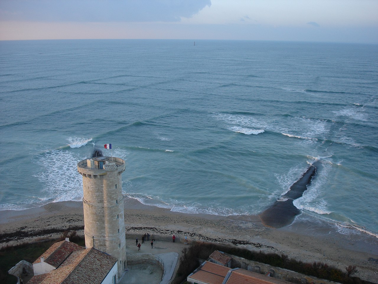 [2] [2] |
By doing this, we can do the following:
- Estimate the underlying variables given the data and the assumed physical model;
- Calibrate a misspecified model in the face of noisy, observed data;
- Predict what the phenomena will look like in the future;
- Quantify the uncertainty of solutions in an interpretable statistical framework.
Application to digital twins
Digital twins are models that contain the physics of a real-world model, for example a PDE, and are continually updated with observed data from the real twin. Digital twins are used for estimation, forecasting and decision making with respect to the physical twin, in a growing list of application fields, such as structural health monitoring, precision medicine, climate modelling, agricultural modelling and oceanography [4]. Digtal twins are characterised by their need to assimilate large quantities of sensor data with underlying physical models with statistical uncertainty; it is clear that a statistical framework is needed to underpin digital twins.
For example, in [5], a digital twin of an instrumented bridge is developed. Sensor data of the strain, that is perhaps noisy and sparse, is assimilated with an assumed, underlying finite element model of the structural mechanics, which may be misspecified, in order to estimate the true strains in the bridge.
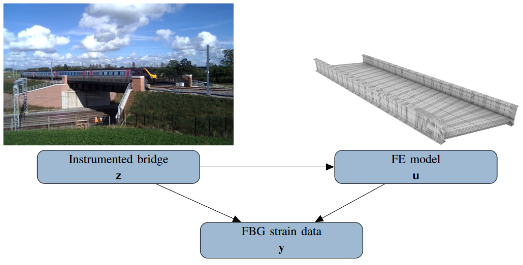 [5]
[5]
Background
The statistical finite element method has been developed in [6] in order to tackle this problem of data assimilation. In their model, data x is observed via an assumed noisy, linear mapping. The data assimilation problem is framed as a Bayesian filtering problem; the likelihood of the data x is combined with a prior arising from the solution of a stochastic PDE (SPDE) to form posterior estimates of the latent (underlying) variable u. In effect, the method solves the SPDE to give a first order linear Markovian state-space model:
where subscripts represent sets of parameters. Then, the filtering posterior is
\[p_{\Lambda, \nu}\left(\mathbf{u}_{1: T} \mid \mathbf{x}_{1: T}\right)\]For example, below, sparsely observed data and an underlying, invisble PDE are combined to give statistical estimates of the posterior.
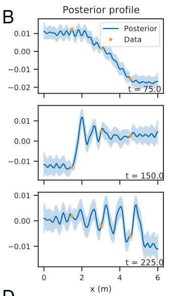 [6]
[6]
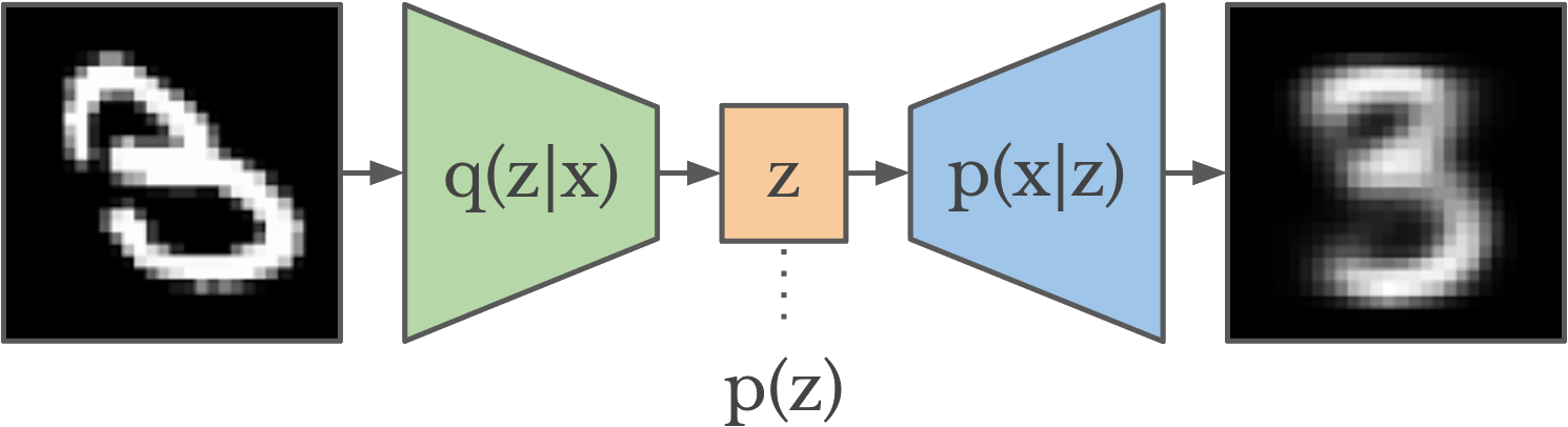
In order to model more complex data, such as image/video data in the wave examples above, we need a way to model and also learn complex data mappings, which are much harder to provide by hand, without knowing already what the solution is meant to be. In the field of machine learning, this is known as unsupervised representation learning. One such approach is the variational autoencoder (VAE) [7] below:
 [9]
[9]
In a VAE, an encoder models dimensionality reduction into a lower-dimensional latent space, and a decoder models the inverse, generative mapping. The latent space “bottleneck” has a prior to enforce an efficient representation space. The neural networks of the model are trained end-to-end in a unsupervised manner, using a variational lower bound of the Bayesian evidence, where y are observed images and x are the latents, the tilde represents a sampling step taken during variational inference and KL means the Kullback-Leibler divergence:
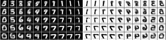
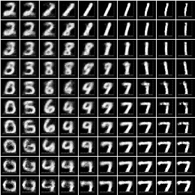
The VAE has been shown to learn meaningful, smooth low-dimensional representations of data…
 [8]
[8]
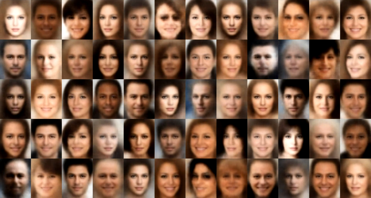
… and also generate synthetic data that is realistic but novel, such as from this VAE trained on human faces:
To start modelling time dependency in the VAE latent space, the dynamical variant called Kalman VAE (KVAE) [10] introduces a linear state-space model (SSM) into the VAE latent space, and infers latent state-space sequences using the Kalman Filter. This is useful as the inferred posteriors are a Bayesian combination of the VAE data and some dynamical SSM. The resulting evidence lower bound combines parameters from both the state space model and the VAE, and combines the variables u (latents), x (pseudo-observations) and y (observations):
where q is a distribution taken from the variational family (usually Gaussian) which is to be optimised.
Our approach
The aim in [10] was to learn the parameters of the linear dynamical model from data. However, our approach instead fixes the parameters according to an assumed SPDE. We can do this because in the linear case, solving a SPDE with statistical finite elements gives a linear transition model. Therefore this transition model can be elegantly “dropped-in” into the KVAE latent space, where the dimension is the number of finite elements. The transition model is calculated to be, in the case of a linear SPDE using the explicit Euler spatial discretisation method:
\[\begin{aligned} p_{\Lambda}\left(\mathbf{u}_n \mid \mathbf{u}_{n-1}\right) & =\mathscr{N}\left(\mathbf{u}_n ; \mathbf{F}_{\Lambda} \mathbf{u}_{n-1}+\mathbf{f}, \mathbf{Q}\right) \\ \mathbf{F}_{\Lambda} & =\mathbf{I}-\Delta_t \mathbf{M}^{-1} \mathbf{A} \\ \mathbf{f} & =\Delta_t \mathbf{M}^{-1} \mathbf{b} \\ \mathbf{Q} & =\Delta_t \mathbf{M}^{-1} \mathbf{G M}^{-\top}\end{aligned}\]where M and A are finite-dimensional matrices representing the PDE in discretised Sobolev space, G is a finite-dimensional diffusion matrix constructed according to the assumptions on the noise, and \Delta_t is the time discretisation constant.
Our model is physics-informed: instead of having to learning dynamics from scratch, inference combines knowledge of the underlying PDE “prior” and the observed data. Note that there are two perspectives here. Firstly, we have equipped a physics model solver with deep feature extraction capabilities that are learnt in an unsupervised manner. Alternatively, we have equipepd a deep representation learning model with dynamics that are informed by physics.
Experiments
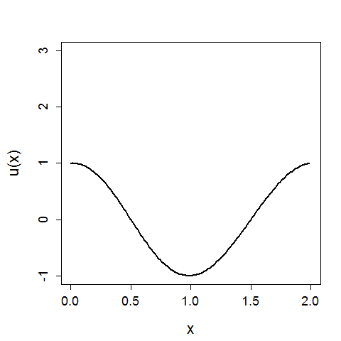
In experiments for this project, we firstly generate a synthetic video dataset from the analytical solution to the 1D wave equation. Even though the dataset is very simple, the mapping is still non-trivial and requires some knowledge of 2D spatial dependency:
Then we solve the wave PDE with statistical finite elements, and fix the KVAE latent space with the resulting transition model. The transition model prior mean should look something like the original wave:
We expect the inferred sequence posteriors to look like a stochastic combination of the mapped dataset and the underlying transition model.
All models are implemented and trained with PyTorch. The encoder and decoder networks are very simple convolutional neural networks (CNNs). The loss function is the negative log-lower bound of the evidence using variational inference, and contains terms relating to VAE reconstruction, VAE regularisation, the stochastic filter log-likelihood and the transition model log-likelihoods. Please see the full report for a full derivation of the model.
Results and discussion
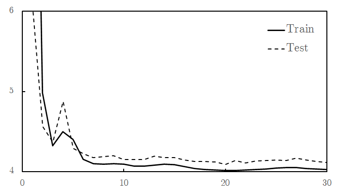
After the model has been trained, we can firstly check for training and generalisation success by plotting the loss function:
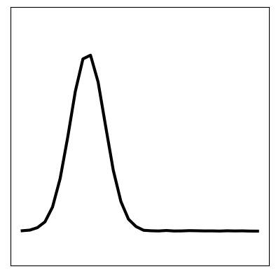
We can also pass a test sample through the model (below left). We see that the image has been successfully reconstruced through the encoder-decoder model (below right). However, most importantly, the inferred latent space sequence (below middle) closely resembles what we expect the underlying variables to be: a vector following the wave equation. This sequence has been inferred from the higher-dimensional data, given knowledge that it should follow the wave equation.


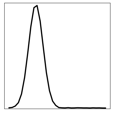
Furthermore, we can set a truthful initial condition in the latent space and propagate forward in time according to the transition model (below left). Then, by passing this through the decoder, we can predict a new sequence in the future that resembles the original seen data (below right):

We can compare these results to the original KVAE from [10] that is uninformed, and instead has to learn dynamics. The same visualisations are reported below. We see that in an uninformed model, it is difficult to learn the correct dynamics, and hence the inferred latent space does not resemble the underlying variables of the wave equation. The reconstruction still looks good; CNNs can learn very non-linear mappings that the dynamics have failed to capture.
With these poorly learnt dynamics, we can’t predict in the future.
References
- [1] [Ta2o](https://commons.wikimedia.org/wiki/File:KdV_equation.gif” alt=”drawing” width=”100%”/>. CC BY-SA 3.0
- [2] [M. Griffon](https://commons.wikimedia.org/wiki/File:Ile_de_r%C3%A9.JPG” alt=”drawing” width=”100%”/>. CC BY 3.0
- [3] [Zureks](https://commons.wikimedia.org/wiki/File:Example_of_2D_mesh.png” alt=”drawing” width=”100%”/> CC BY-SA 3.0
- [4] Scaling digital twins from the artisanal to the industrial. Niederer et al., 2021.
- [5] From Digital twinning of self-sensing structures using the statistical finite element method. Febrianto et al., 2021.
- [6] Statistical finite elements for misspecified models. Duffin et al., 2020.
- [7] Auto-Encoding Variational Bayes. Kingma and Welling, 2014.
- [8] Wojciech Mo. Accessed 02/06/2022.
- [9] Danijar Hafner. Accessed 02/06/2022.
- [10] A Disentangled Recognition and Nonlinear Dynamics Model for Unsupervised Learning. Fraccaro et al., 2017.